Figure 1. Directional Bridge Terminated with 50 Ohm Pad
Figure 2. Return Loss of Double Ridge Horn #1
Figure 3. 1 - 2 GHz discone
Figure 4. 2 - 4 GHz Discone
A Different Antenna for the Mode-Stirred Chamber |
Matthew R. Wills
|
Directional antennas are a necessary part of RF susceptibility testing because of a need to direct the RF energy toward a specific EUT using a spot illumination methodology. In the case of the mode stir chamber (MSC) the antenna serves as a transducer to transfer the energy into the chamber. Directional characteristics are not needed. In this case the antenna chosen was the discone antenna. The discone will be compared to a double ridge horn from the standpoint of return loss. These simple antennas improved the return loss from –5dB to better than –10dB and eliminated transmit antenna changes during a test. The discone antenna efficiency is within 1dB of the double ridge horn based on test field strength measurements. The reflected energy from the double ridge horn antenna was sufficient to activate SWR (Standing Wave Ratio) shutdown circuitry in the TWT (Traveling Wave Tube) amplifiers thereby limiting the forward power available from the amp.
At some test frequencies, the amp would shut down completely from a high SWR condition. Other labs attribute the TWT shutdown to energy return from the chamber, in our mode stir chamber the return at 1 GHz is over 10dB down. The discone antenna has better SWR characteristics across the frequency range of interest and may be constructed easily by the user. This article will have some technical detail and will provide construction details in a “this is how I done it” fashion.
During the first year of operation of the Cessna mode stir chamber, we had a power limitation on the receive antenna. The dipole used from 100 – 250 MHz was rated 10 watts max. This required that chamber calibrations be done at the 10W level and cal levels scaled up to the test levels.
In the mode stir chamber the insertion loss may be quite small at low frequencies.
A discone receiving antenna was purchased at a nationally known electronics
store and tested for use as a receiving antenna (100 -1000 Mhz). The antenna
has been in continuous service since. During the initial testing of the discone,
the 50W attenuator connected to the antenna was overheated and destroyed due
to low insertion losses. 100W attenuators are now the minimum used. This is
from an antenna with a cost of less than $75, and the reality is, it fills the
job very well. Test calibrations are now performed at the full test levels.
This prompted us to look at discone transmit antennas for the higher frequencies.
The horn and the discone antennas were compared using an HP-85025C Directional Bridge, HP-83620A RF Sweeper and an HP-8757D Scalar Analyzer.
The bridge was operated into an open circuit and a calibration level stored,
this represented a 0 dB return loss. Next the antenna to be tested was placed
on the bridge and a sweep taken over the band of interest. The charts produced
indicate return loss in dB.
The goal for the discone antenna was to obtain < -10 dB return loss. The antennas were not tested in any special environment, simply in an open lab area. Reflections did not seem to influence the return loss measurements to an intolerable level. These tests could be repeated in more controlled conditions to improve uncertainties from range reflections.
|
|
Figure 1. Directional Bridge Terminated with 50 Ohm Pad |
Figure 2. Return Loss of Double Ridge Horn #1 |
|
|
Figure 3. 1 - 2 GHz discone |
Figure 4. 2 - 4 GHz Discone |
|
|
Figure 5. 4 - 8 GHz Discone |
Test results show that the discone return losses were always equal to or better than the double ridge horn over equivalent frequency ranges as shown in Fig 1-5. In some frequency bands, the discone is much better. A high-pot test was tried at 1000 Volts with no apparent problems.
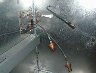
We have been pleased with the performance of the discone antennas. We are currently using 4 separate discones from 1 to 8 GHz. Examples of the discone and horn antennas are shown in Fig 6. Fewer antennas could have been used, but it is more convenient to have a separate antenna connected to each TWT amplifier.
 |
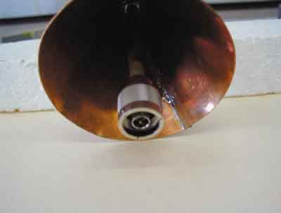 |
Figure 6. 1 to 18 GHz transmit antennas (1 - 8 GHz discones, 8 - 18 GHz Horn) |
Figure 7. Construction Photo #1 |
 |
|
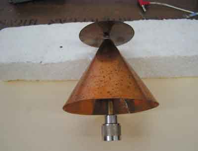
Figure 8. The finished antenna, ready for installation. |
Construction time is about 8 hours.
The antennas were constructed using a crimp on connector, brass tubing from
a hobby store and copper sheet. Silver solder would be nice for some of the
joints but is probably not a requirement.
The outer conductor for the feed line is made from brass tubing with a .282 inch inside diameter. The inside conductor is made from 1/8 inch brass tubing. Using the air dielectric transmission line formula,
d1 = inside diameter of the outer conductor
d2 = outside diameter of the inner conductor
Zo = 48.76 ohms, fairly close to the required 50 Ohm impedance.
The cone of the discone is made by cutting a half circle of copper to the required radius plus 1/4” overlap on the edges for soldering. The edges are brought together and soldered. The top of the cone is then cut away to allow a slip fit onto the outside diameter of the transmission line section and soldered in place. See Fig 7 and 8.
The first discone was built using 5/8 inch copper tubing as the XMSN line. There seemed to be a lot of ripple in the return loss response. Changing over to the smaller tubing reduced the ripple. The transmission line is soldered into a coaxial crimp connector that has had a hole bored into it the same size as the outside of the transmission line. The hole must fit fairly tightly. This joint would be best if it were silver soldered for the extra strength. Soft solder will work though.
The center pin of the coax connector is soldered to the center conductor of the transmission line using a short piece of wire that fits the center pin and is in turn soldered inside the 1/8 inch tubing.
The following formulas were used to determine sizes for discone. A search for discone antennas on the Internet will yield several resources. Don’t forget your local ham radio operators, this is right up their alley!
When designing for a specific frequency band, use a frequency about 20% below your desired start frequency. This will improve the low-end characteristics. The discone theoretically has a 10:1 frequency range, but for lower SWR, 3:1 is a better number based on our results. This fits well with the octave range of the TWTs.
FMHz = Frequency in megahertz
Dimensions are in inches.
L = length of the cone in inches
D = diameter of the top disc in inches
S = distance from the top of the cone to the disc in inches
In practice, it is easier to leave the center conductor a little long and trim it to adjust the spacing between the disc and the top of the cone, by measuring the return loss.
 |
Matthew Wills has been employed as an Engineering Technologist by the Cessna Aircraft Company in Wichita, Kansas for the last seven years. For the last five of these, he has been with the Electromagnetic Effects Lab. Prior to working for Cessna, he was employed for two years in television broadcasting, five years as an avionics bench technician and five years as an electronics instructor. He graduated from the Wichita Technical Institute, Wichita, Kansas in 1982. He is married with one daughter. He may be reached at phone 316-831-2631 or via e-mail at mwills@cessna.textron.com.EMC |
© Copyright 2001, IEEE. Terms
& Conditions. Privacy
& Security