 |
Figure 1. |
Arthur J. Glazar, P.E.,
Life Senior Member,
IEEE
Abstract - In 1977, Albert A. Smith, Jr., first published "Coupling of External Electromagnetic Fields to Transmission Lines". Smith analyzed the coupling mechanism between ambient electromagnetic (EM) fields and a transmission line (TL), and formulated a suite of equations broadly applicable to the prediction of radiated susceptibility (RS) of various wire and cable configurations. Smith's seminal book, and the expanded 1987 second edition, provides many practical worked-out examples and spectrum profiles. The present author, however, needed specific solutions to a cable susceptibility problem and therefore undertook the task of implementing a subset of Smith's equations for use on a personal computer. The end result is the subject of this paper: a simple-to-use program designed to quickly evaluate the RS of shielded cables above perfect ground in typical applications. The program (COAX.EXE) generates solutions in graphic format, displaying load current or voltage spectra resulting from four different EM field orientations, and it facilitates parameter variations such as cable length, height above ground, terminating impedances and coax characteristics. Using COAX.EXE, the author was able to closely replicate several problem solutions published by Smith, thus lending confidence to the code. COAX.EXE is compact and will run on minimally-configured personal computers. It is available as freeware to EMC Society members and others.
The EMC engineer's toolkit typically comprises textbooks, clipfiles, software, and most importantly, his own knowledge acquired from prior experience. Although software has become increasingly important, it has been the author's experience that software is often too generalized and overly complex, or just too expensive or otherwise inaccessible.
One frequently-encountered EMC problem is that of predicting the radiated susceptibility (RS) of box-to-box cabling. Whenever a system incorporates cabling interconnection, the question of RS must be addressed whether or not a formal specification exists. Credible RS prediction tools can help to avoid the need to rework and retest a design. In those instances when formal analysis is required, confidence is enhanced if a mathematically-defensible solution can be obtained, rather than an extrapolation from a similar application.
This paper discusses the author's software implementation of a subset of the equations developed by Albert A. Smith, Jr.[1]. The software allows the user to set up a circuit consisting of a coaxial cable whose shield, as well as its signal-carrying center conductor, can be terminated in complex impedances at both ends. The cable is positioned above, and parallel to, a perfect ground plane, and is illuminated by a uniform electromagnetic field. After the user enters various problem parameters, the program displays graphical solutions of the load current (or voltage) spectrum over six decades of frequency, from 10 Khz to 10 Ghz. Graphical solutions are provided for each of four field orientations.
In setting up a problem, the user is prompted for problem-definition parameters. Possibly the most significant of these is the surface transfer impedance, Zt of the coaxial (or other shielded) cable. In the past, specifying Zt in a useful way has been difficult. The present program, however, reduces that task to simply choosing one of seven stored functions, or to generating a customized function by entering a series break of frequencies and magnitudes.
The foregoing is best illustrated by studying Figures 1, 2 and 3 which are screen captures obtained while running the following example problem: A one-meter length of RG-58/U connects two ideal system boxes. The cable is supported 0.1 meters above ground and subjected to a 100 v/m, horizontally-polarized field. The source end of the signal-carrying center conductor is terminated by 50 + j0 ohms, and the load end by 50 ohms in parallel with a capacitive reactance of -15,900 ohms at 1 MHz (i.e., 10 pF). At both ends, the coax shield is terminated to ground by a pigtail connection which is simulated as a series-connected 0.1 ohms and +3.14 ohms of inductive reactance at 1 MHz (i.e., 0.5 microhenries). Figure 1 is the DATA ENTRY menu showing all of the problem parameters; Figure 2 is the TRANSFER IMPEDANCE SELECTION screen, from which Curve #1 (RG-58/U) has been selected. Figure 3 is the problem solution graph.
|
Figure 1. |
 |
Figure 2. Transfer impedence selection screen for the example of Figure 1. |
Part II of this paper reviews transmission line (TL) coupling theory, and Part III discusses the features and limitations of the software.
 |
Figure 3. The problem solution graph for the example of Figure 1. |
TL theory treats the outer shield (sheath) of a coaxial cable as a conductor above a ground plane, which forms a uniform, lossless transmission line. Such a transmission line has a real characteristic impedance equal to
Zo = 138 Log10 (4h/d)
where
h = shield height above ground,
d = shield diameter
d, h in consistent units
The end points of the shield are terminated at the ground plane in impedances ZS1 and ZS2 which may be complex. Figure 4 illustrates the shield and signal terminations. For TL theory to be valid, the shield height, h, must be small compared to the line length and also must be a negligible fraction of a free space wavelength.
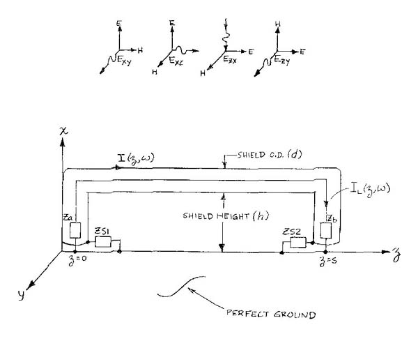 |
Figure 4. |
As far as the signal-carrying portions of the coaxial cable are concerned, the interior characteristic impedance of the coax will be denoted as Zc to distinguish it from Zo. Also, the signal-carrying center conductor is terminated in complex impedances Za and Zb, representing the source and load ends of the signal circuit, respectively.
If this configuration is illuminated by an electromagnetic field having a component parallel to any portion of the shield, current will flow on the surface of the shield. Because the shield is imperfect, the surface current will couple into the center conductor (i.e., into the signal circuit) of the coaxial cable. The mechanism for this coupling between shield and signal circuit can be described by a function known as the surface transfer impedance, Zt, of the cable. This function has the dimensions of ohms per unit of cable length along the z-axis, and is defined by the differential equation
dV(z) = Zt I(z) dz
This definition implies that a differential voltage is generated in the interior of the cable, which voltage is proportional to the shield surface current, I(z) and the magnitude of Zt. It is this differential voltage along the center conductor that causes an undesired component in the signal load. It should be noted that Zt is also frequency dependent, and in practice is usually a measured parameter and is presented as a plot of impedance magnitude vs frequency.
Figure 4. illustrates the E-field notation used by Smith [1] and adopted herein. The four fields shown are those which provide maximum coupling into the cable system defined in Figure 4. All are assumed to be uniform, transverse plane wave fields. Ex(y) represents a vertically-polarized field traveling in the y, or -y, direction (broadside incidence). Ex(z) represents a vertically polarized field travelling in the z, or -z, direction (end-fire incidence). Ez(x) represents a horizontally polarized field traveling in the -x direction; that is, propagating from directly overhead toward the ground plane (edge-fire incidence). Finally, Ez(y) represents a horizontally polarized field traveling in the y, or -y direction.
Note that two additional horizontally-polarized fields Ey(x) and Ez(x) would be orthogonal to all parts of the conductor system defined in Figure 4, and no coupling would occur. Also, Ex(x), Ey(y) and Ez(z) are not physically realizable fields since transverse electromagnetic (TEM) waves can have no field component in the direction of travel.
Ez(x) requires additional comment. Of the four fields being considered, it is the only one wherein the total field in the vicinity of the conductors may be different from the incident field. If we assume that an Ez(x) field having an incident magnitude, Ei, was launched from some large distance above the ground plane, it would encounter the ground plane and experience total reflection at the surface of the plane. The net result would be a standing wave producing a total field having a magnitude of zero at the ground plane and at even-multiples of a half-wavelength above ground. Similarly, the total field would have a magnitude of 2 Ei at odd-multiples of a quarter wavelength above ground; that is, Ez(x) = 2 Ei sin 2ph/l. In a test chamber or in any other real environment, a cable system will respond to the total field, which can be vastly different from the incident field. At any given frequency and height above ground, this difference can range from a +6dB increase to an infinitely deep null response.
Smith [1] showed that a current IL(z,w) will flow in the signal load, Zb, due to a current distribution, I(z,w), along the length of the shield:
 |
where:
P = Zc (Za + Zb) cos bi s + j(Zc2 + Za Zb) sinbis
Za = coax signal source terminating impedance, Ra + j Xa
Zb = coax signal load terminating impedance, Rb + j Xb
Zc = coax internal characteristic impedance, ohms
w = radian frequency = 2 p f
f = frequency, Hz
z = distance along cable, meters
Zt = surface transfer impedance, ohms/m
bi = coax internal wave number = bVf
b = free space wave number = w / c
Vf = coax velocity factor
c = 3 x 10⁸ m/s
s = cable length, meters
For Ex(y):
I(z,w) = K1 {Zw [cosb(s-z) - cos bz] + j[Z2 sinb(s-z) - Z1 sin bz]}
For Ex(z):
I(z,w) = K1 [ (Zw - Z1) sinbs sinbz + j(Zw + Z2) sinbs cos bz - j(Z1 + Z2) cos bs sinbz]
For Ez(x):
I(z,w) = K2 [1 - (N1 + jN2) / D]
For Ez(y):
I(z,w) = K3 [1 - (N1 + jN2) / D]
where:
Ei = Incident electric field strength, V/m
h = shield height above ground, meters
d = shield diameter, meters
Zw = 2 Zo = 276 Log10(4h/d)
ZS1, ZS2 are the shield terminating impedances at ends 1,2 respectively
Z1 = 2 ZS1 = 2 (RS1 + jXS1)
Z2 = 2 ZS2 = 2 (RS2 + jXS2)
D = Zw (Z1 + Z2) cos bs + j(Zw2 + Z1 Z2) sinbs
K1 = 2 h Ei /D
K2 = (2 / Zw b) (2 Ei sin 2ph/l)
K3 = (2 / Zw b) (Ei)
N1 = Zo Z2 cos bz + Zo Z1 cosb(s-z)
N2 = Z1 Z2 [sinbz + sinb(s-z)]
It is evident that paper-and-pencil solution for any specific set of parameters would be a formidable undertaking.
Implementing equations was a straightforward programming
task, but developing a simple and intuitive user interface required careful consideration.The
following discussion addresses some of the considerations and their resolution.
Plot Display. Solutions are plotted in semi-log format. The frequency range is
fixed at six decades (10 Khz to 10 Ghz), and the magnitude range is fixed at 200
dBv or dBa. Automatic range scaling was initially considered but found to be un-necessary
because the dB range becomes evident after the first pass and the user can shift
the dB scale up or down as necessary. The default range is ±100 dB. The user can
also select either load voltage (dBv) or load current (dBa) for presentation.
The display utilizes 300 pixels across the frequency axis; i.e., 50 pixels per decade, to achieve maximum plot resolution. During a plot, the program assigns these pixel numbers as the independent variable, and frequencies are calculated as a function of pixel number. Since the plot comprises 300 discrete frequencies, it is possible that a particular plot feature (a cusp, for example) may fall between two frequencies and thus fail to present a true maximum or minimum. In such cases, the user can "zero in" on the true frequency and amplitude by selecting a "frequency multiplier" factor from the data entry menu. The allowable multiplier range is ± 1% (0.99 to 1.01). When the multiplier is within that range (but not unity), the plotting routine goes into single-step mode and all frequencies are multiplied by the selected factor. By this means, the frequency and amplitude of any plot feature can be evaluated.
Complex Loads. From the data entry menu, the user can select terminating impedances for both the shield and the signal line. The allowable impedance choices are series-connected or parallel-connected resistance and reactance. Reactance values are specified at 1 MHz, and may be either capacitive (negative) or inductive (positive). The data entry menu requests the user to prefix the resistive value with a "p" for a parallel R-X connection; otherwise the default configuration is series connection. The program makes the necessary impedance transformations during problem execution. This particular scheme for designating impedance may be unorthodox, but the author found it convenient and intuitive. The terminating impedance values and all other problem input parameters appear at the top of the solution plot for reference.
Transfer Impedance. The transfer impedance selection screen enables the user to synthesize any Zt curve. Building the curve is an interactive process. The program repetitively asks for break frequencies and dB values and continuously displays the construction of the curve. Any number of frequencies between 10 kHz and 10 Ghz can be employed to create a piecewise linear curve to any degree of smoothness desired, up to 100 breakpoints. The program offers no means to store user-generated Zt curves. Figure 2. shows the Zt selection screen and identifies the seven available curves which are approximations derived from several different sources.
Coaxial Cable Parameters. Figure 1 reveals that three coaxial cable parameters must be provided by the user. These are (a) characteristic impedance; (b) velocity factor; (c) shield outside diameter. For convenience the program includes a short table of common coaxial cable types with these parameters. The table is reproduced in Figure 5.
 |
Figure 5. |
About the Program. COAX.EXE was written and compiled using Microsoft's (R) BASIC version 7.1 Professional Development System. This DOS-based software includes the QuickBASIC Extended (QBX) development environment which has served the author for numerous engineering applications. COAX.EXE is a modest 80 kilobytes in length, requires only minimal memory and no installation. VGA is required, but a color monitor is optional. Maximum execution speed is obtained by running directly from DOS. Execution time for a typical plot was timed at 40 seconds when run under DOS from diskette on a 486 DX33 computer. The program has no provision for hardcopy or for saving problem data. All computation is done "on the fly". The program's introductory screen offers the user the option of switching to a white background which is better suited to printing a screen. If the program is run under WINDOWS, a screen image can be captured (cut) by pressing Alt+PrintScreen, then pasting into an accessory program such as PAINT or WORDPAD, from where it can be printed.
Program Availabilty. COAX.EXE is available directly from the author at aglazar@ieee.org.
[1] A. A. Smith, Coupling of External Electromagnetic Fields to Transmission Lines, second edition, Interference Control Technologies, Inc., Gainesville, VA (1987).
 |
Art Glazar obtained his B.E.E. degree from Pratt Institute in 1960, P.E. Certification in 1977, and retired from industry in early 1991. His last position was with Loral Fairchild Systems in Syosset, NY, where he was responsible for EMC analysis and compliance for the USAF ATARS program. He can be reached by telephone at 631-724-1520, and email at aglazar@ieee.org .