Radio Disturbance Measurement and its Uncertainties

By Stephane Laik

Introduction

The EC labelling of electronic equipment to be made available on the European market makes it necessary to carry out EMC tests with a view to satisfying the basic requirements of directive 89/ 336/EEC. In particular, this directive imposes the determination of the level of emission of disturbances radiated by the equipment and its comparison with a limit which must not be exceeded. To respect these requirements, it is important to know the measuring method used and the uncertainties associated with it.

Mathematical model

When making measurements on an equipment item, it is necessary to know all the characteristics of the measuring system used. For example, to measure the electric field radiated by a device, the setup used is similar to that described in figure 1.

In this case, the electrical field measured can be expressed as:

E(µV|m)=V(µ).k(m^-¹).P.(1+D) or

E(dBµV|m)=V(dBµV)+ K(dB|m)
+ P(dB)+D(dB)

with: V, the measurement given by the apparatus   

k, the antenna factor

P, cable losses   

D, uncertainties connected with impedance mismatches.

Figure1: Measurement setup.

In the 30 – 1000 MHz frequency band, two types of antennas are often used: a biconical one between 30 and 200 MHz and a log-periodic one between 200MHz and 1000 MHz.

Parameters influencing measurement

The measurement recorded is influenced by elements inside and outside the measuring system. [NIS81] proposes a non-exhaustive list of these parameters : Ambient signal, Antenna factor calibration, Cable loss calibration, Receiver specification, Antenna directivity, Antenna factor variation with height, Antenna phase centre variation, Antenna factor frequency interpolation, Measurement distance variation, Site imperfection, Mismatch impedance, System repeatability.

It is possible to put a numerical value on these uncertainties in most cases. The simplest method is to calculate the overall uncertainty on the bandwidth under consideration by taking the maximum value of all the partial uncertainties. But this method has the disadvantage of giving a result that does not really reflect the measurement. It is wiser to calculate the uncertainty per frequency band, dividing up the bands as fixed by the calibration certificates. In this case we obtain:

• Antenna factor calibration uncertainty (Probability distribution : normal, k=2)

    30 to 100 MHz  Þ  ± 1.1 dB

    100 to 200 MHz  Þ  ± 0.9 dB

    200 to 600 MHz  Þ  ± 1.0 dB

    0.6 to 1 GHz  Þ   ± 1.2 dB

• Antenna reflection coefficient uncertainty (Probability distribution : normal, k=2)

    0 to 0.2  Þ ±  1.1 dB

    0.2 to 0.4  Þ ± 0.9 dB

    0,4 to 0.6  Þ ± 1.0 dB

    0.6 to 0.8  Þ ± 1.2 dB

    0.8 to 1  Þ  ± 1.2 dB

Comparing these data with the calibration results (Figure 2 to Figure 5) we obtain the following six divisions:

30 to 45 MHz (Biconical antenna, G > 0.8)

45 to 85 MHz (0.8 > G > 0.6)

85 to 100 MHz (0.6 > G > 0.4)

107 to 200 MHz (0.4 > G > 0.2)

200 to 600 MHz (Log-periodic antenna, 0.4 > G > 0.2)

600 to 1000 MHz (G < 0.2)

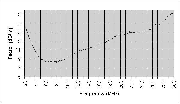Figure 2: Biconical antenna factor

Figure 3: Log-periodic antenna factor

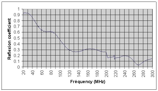Figure 4: Biconical antenna refexion coefficient

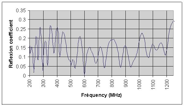Figure 5: Log-periodic antenna reflexion coefficient.

Table 2 lists all the uncertainties per frequency band. From these uncertainties it is possible to calculate the standard uncertainty on the measurement of radiated disturbances. In the first band we obtain:

The expanded uncertainty for a 95 % confidence level in the measurement is: U = 2U_c = 5.26 dB.

The uncertainty calculation on mismatches is given by: U=20log(1±G_lG_g) where G_g, is the reflection coefficient of the antenna and G_l = 0.3 is the reflection coefficient of the measuring receiver.

Table 2: Uncertainty budget

Interpretation of calculations

Once the characteristics of the measuring system are known, it only remains to take the measurements on the equipment item

Case A	Case B	Case C	Case D
The product complies.	The measured result is below the specification limit by margin less than the measurement uncertainty. It is not therefore possible to determine compliance at alevel of confidence of 95%. However, the measured result indicates a higher probability that the product tested complies with the specification limit.	The measured result is above the specification limit by a margin less than the measurement uncertainty. It is not therefore possible to determine compliance at a level of confidence of 95%. However, the measured result indicates a higher probability that the product tested does not comply with the specification limit.	The product does not comply.
Table 1. Compliance Criteria (NIS 81)

and compare them with the upper limit fixed. The four possible cases are shown in table 1.

Application to measurement on free field site

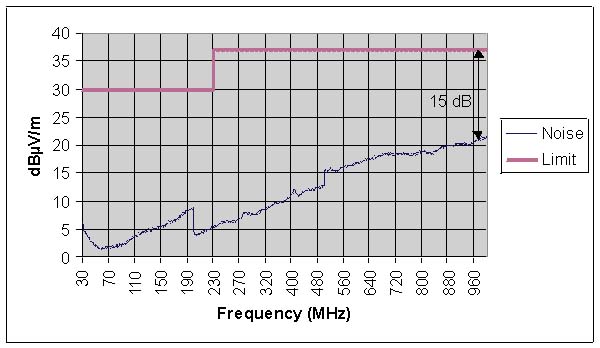
In the case of free field site measurements on a class B equipment item, standard NF EN 55022 (CISPR 22) sets the upper limits at 30 dBµV/m between 30 and 230 MHz, and 37 dBµV/m between 230 and 1000 MHz. Figure 6 compares the noise levels of the measuring system over the whole frequency spectrum.

It can be seen that around 1 GHz the difference between the standard and the noise level of the measuring system is 15 dB (Figure 6). For compliance at a level of confidence of 95%, the maximum radiation must be 3.69 dB below the limit in order to fall into case A of Table 1, i.e. its radiation level must be 33.31 dBµV/m. In these conditions, the signal/noise ratio is 11.31 dB and the measurement indicated suffers from additional error. Figure 7 shows how the error on the measurement indicated by the receiver increases with the signal/ noise ratio. With a signal/noise ratio of 11 dB, the uncertainty on the measurement rises from 3.69 to 4.93 dB and we find ourselves in case B of Table 1.

It is, however, possible to remove the ambiguity for sine-wave signals while respecting the spirit of the standard by reducing the pass band of the filter (fixed at 120 kHz). With a 9 kHz filter, the noise level drops 20 dB or so and the signal/noise ratio increases in consequence. This only gives correct results if one and the same signal is present in the pass band of the 120 kHz and 9 kHz filters. If this is not the case, the total energy of all the signals included in the 120 kHz pass band will be higher than the total energy of all the signals included in the 9 kHz pass band and the bandwidth reduction will result in a reduction of the radiated disturbance measurement, thus giving a rather over optimistic ruling on the compliance of the product.

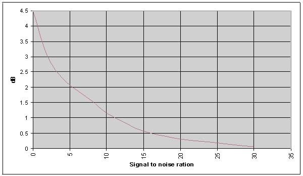Figure 6: Noise level of the measurement method	Figure 7: Error indication

Conclusion

In this article we have highlighted the importance of knowing and qualifying all the elements of a measuring system perfectly if false conclusions as to the acceptability of the equipment under study are to be avoided. We have pointed out the influence of the pass band of the filters on the quality of the measurement intended to determine whether the equipment complies with standard NF EN 55022 but only for cases of emission of isolated sine-wave signals. For wide-band pulse signals there are no methods for giving so simple a ruling without completely distorting the spirit of the standard since other parameters such as the signal repetition frequency and the quasi-peak detector response must be taken into account.

References

NF EN 55022 : Limits and methods of measurement of radio disturbance characteristics of information technology equipment – January 1999.

NIS 81 : The treatment of uncertainty in EMC measurements– 1st edition May 1994

Stephane Laik received a DEA diploma in electronics, with a specialty in microelectronics systems, from the University Paul Sabatier in Toulouse, France in 1994. He is currently working on his Ph. D. thesis at Ecole Doctorale de Genie Electrique, Electronique, Telecommunication in Toulouse. (Jean-Louis Boizard is his thesis advisor.) He is also working in a COFRAC-accredited EMC laboratory at Societe de Construction de Lignes Electriques (SCLE). His research interests include EMC tests for improving electronic design. Stephane can be reached via e-mail at slaik@club-internet.fr.

Jean Louis Boizard received a Ph. D. degree in Automatic Control from the Universite Paul Sabatier in Toulouse, France in 1985. His research was on three dimensional vision systems based on the use of CCD cameras for robotic applications. He has worked as a project manager on the design of electronic systems for spatial, aeronautic and automotive applications, and is currently an assistant professor at the Institut Universitaire de Formation des Maitres (IUFM) in Toulouse. His present research activities, with the Laboratoire d'Acoustique de Metrologie et d'Instrumentation (LAMI) of Toulouse, include signal processing architectures for wide band acoustic antennas and EMC modeling for CAD tools. Dr. Boizard can be contacted via e-mail at boizard@cict.fr. EMC

Return to Table of Contents

Go to: Penetration of Electromagnetic Fields Through Shielding Barrier Material